Parameter Sweeps and Walk-Forward Analysis

The trap chapter 9 didn’t warn you about#

Chapter 9 showed one way a backtest report can lie to you: a headline number, like a triple-digit Sharpe ratio, that looks spectacular purely because the sample behind it was too short or too suspiciously smooth to deserve that much confidence. There’s a second, more dangerous way the same lie shows up — one that a systematic trader will walk straight into, not by accident, but by doing exactly what seems like the responsible, rigorous thing: searching many parameter combinations for the best one.

A sweep is nothing new, just many of the same thing#

Start with what a “sweep” actually is, because it’s less than it sounds like. It isn’t a different kind of simulation — it’s Chapter 8’s deterministic Backtest object, run many times, once per parameter combination, with the results collected:

class BacktestSweep<C>(
    private val configs: List<Pair<String, C>>,
    private val backtestFactory: (label: String, config: C) -> Backtest,
    private val parallelism: Int = 1,
) {
    fun run(): SweepResult<C> =
        SweepResult(configs.map { (label, config) -> SweepRun(label, config, backtestFactory(label, config).run()) })
}

Nothing here is a new simulator or a shortcut. Every single point in a sweep is its own fully deterministic, independently reproducible backtest — everything Chapter 8 built still applies to each one individually. A sweep is just many honest questions asked in a row: “how would EMA periods 5-and-21 have done? How about 9-and-21? 13-and-34?” Sort the results and you find the winner. So far, so reasonable.

Why “the winner” can be a coin that never existed#

Here’s the trap, and it’s worth building from a simple example first. Flip 200 ordinary, fair coins twenty times each. Purely by chance, a handful of them will land heads fifteen or more times in a row of twenty flips — not because they’re special coins, but because you ran two hundred independent trials, and some trial landing on an unusual streak is exactly what you’d expect from ordinary randomness at that scale. Pick out the coin with the best streak and call it “the good coin,” and you’ve fooled yourself with pure statistics, not discovered anything real about that coin.

A parameter sweep run against one fixed slice of historical data is structurally the identical experiment. Run enough independent “how would this parameter set have performed” trials against the same historical noise, and some of them will look amazing purely because they happened to fit that particular slice’s specific ups and downs — not because the underlying trading idea is actually good. This has a name: curve-fitting, or overfitting — tuning a strategy’s numbers until they hug the exact bumps of one historical dataset, rather than capturing something that would hold up on data the tuning never got to see.

I ran this for real, sweeping the momentum example’s two EMA periods across six combinations against the same short, clean synthetic price series from Chapter 9:

$ qkt sweep momentum_sweep.qkt --from 2024-01-15 --to 2024-01-16 \
    --param emaFast=5,9,13 --param emaSlow=21,34 --rank sharpe ...

rank  sharpe        trades  totalPnL      label
1     455.50328912  1       140.00000000  emaFast=5,emaSlow=21
2     437.35609431  1       132.00000000  emaFast=9,emaSlow=21
3     428.30589970  1       128.00000000  emaFast=5,emaSlow=34
4     419.26342642  1       124.00000000  emaFast=13,emaSlow=21
5     410.22249156  1       120.00000000  emaFast=9,emaSlow=34
6     392.11912712  1       112.00000000  emaFast=13,emaSlow=34

Every single one of these six configurations reports an outrageous Sharpe over 390 — the same too-clean, too-short-sample illusion Chapter 9 walked through, now happening six times at once. The sweep didn’t fix that problem. It made it worse: instead of one inflated number to be suspicious of, you now have six, and the tool will happily hand you the single most-inflated one and call it the winner. A trader who stops here — sweep, sort, pick the top row — has just built a very elaborate, very confident-looking way to select noise.

Watching one fold happen, start to finish#

The defense against this has a name — walk-forward analysis — but rather than explain the whole mechanism in the abstract, let’s watch it happen once, on one real fold, with real numbers, before generalizing to the full rolling process.

My synthetic price series has three legs: BTC climbs for 40 minutes, falls for 40, then climbs again for 45. Take a 40-minute slice from the middle of that — 00:40 through 01:20, which lands entirely inside the falling leg — and hand it to the same six-config sweep as before:

$ qkt sweep momentum_sweep.qkt --from 2024-01-15T00:40:00Z --to 2024-01-15T01:20:00Z \
    --param emaFast=5,9,13 --param emaSlow=21,34 --rank sharpe ...

rank  sharpe  trades  totalPnL  label
1     —       0       0.00000000  emaFast=5,emaSlow=21
2     —       0       0.00000000  emaFast=5,emaSlow=34
3     —       0       0.00000000  emaFast=9,emaSlow=21
4     —       0       0.00000000  emaFast=9,emaSlow=34
5     —       0       0.00000000  emaFast=13,emaSlow=21
6     —       0       0.00000000  emaFast=13,emaSlow=34

Every configuration ties at zero trades. This isn’t a bug — it’s the strategy behaving correctly. The strategy only ever buys, never shorts, and this 40-minute window is a straight decline; a “buy when the fast average crosses above the slow one” signal simply never fires during a pure downtrend, no matter which two periods you pick. With nothing to distinguish them, the sweep can’t rank these six configurations by performance at all — it falls back to picking whichever one was listed first, emaFast=5, emaSlow=21. That’s a real, honest limitation worth sitting with for a second: sometimes a training window just doesn’t contain the information needed to prefer one parameter set over another, and the tool has to say so rather than pretend it found a winner on merit.

Here’s the discipline: that configuration is now frozen. Whatever training window comes next, no further tuning happens on this fold. The next 20 minutes — 01:20 through 01:40, a stretch of history this parameter search never looked at — is where it gets graded, alone, exactly as-is:

$ qkt backtest momentum_sweep.qkt --from 2024-01-15T01:20:00Z --to 2024-01-15T01:40:00Z \
    --param emaFast=5 --param emaSlow=21 ...

Trades:           1
Final unrealized: 40.00000000
Sharpe (annual):  413.44491801

Something real happens this time. That 20-minute window is the start of the third leg — a fresh uptrend — and the frozen configuration correctly catches the golden cross and buys into it, landing a genuine, non-zero, well-defined Sharpe on data it had zero say in choosing. This is the entire idea of walk-forward analysis in miniature: the parameter search’s job ends the moment training ends, and everything that happens next is graded on ground the search never got to stand on.

Naming the two halves: in-sample and out-of-sample#

The 00:40–01:20 window above is called the in-sample period — abbreviated IS in the report you’ll see next — the stretch a parameter search is allowed to look at while deciding a winner. The 01:20–01:40 window is the out-of-sample period — OOS — a stretch it never saw, used only afterward to grade the one winner already locked in. Every fold in a walk-forward run repeats exactly the two steps just walked through by hand: sweep on the in-sample window, freeze the winner, grade it once on the out-of-sample window.

Rolling that same fold forward through history#

One fold proves very little on its own — it’s one 20-minute grade, and Chapter 9 already showed how little a single short sample can be trusted. Walk-forward analysis repeats the whole two-step process over and over, sliding both windows forward through time by a fixed step, so the same discipline gets applied many times against genuinely different stretches of history:

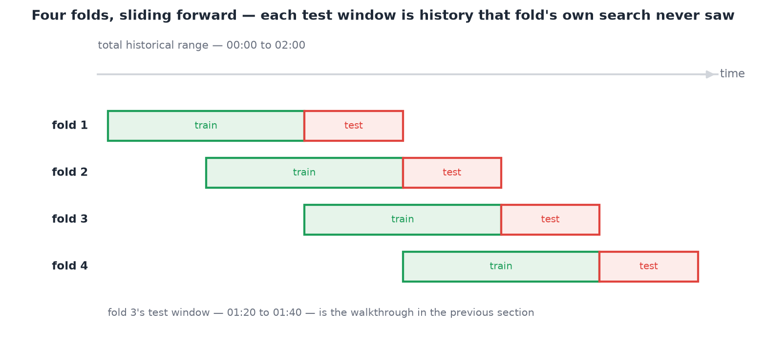Figure 10.1 — Train windows overlap on purpose; test windows never do. Fold 3’s test window is the exact 20 minutes walked through by hand above.

internal fun rollingWindows(total: TimeRange, trainSize: Duration, testSize: Duration, stepSize: Duration)
    : List<Pair<TimeRange, TimeRange>> { /* slides trainStart forward by stepSize each iteration */ }

Notice the train windows overlap between consecutive folds — that’s step being smaller than the train window, and it’s deliberate: fold 2 doesn’t start where fold 1’s train window ended, it starts a little into fold 1’s training period, so each new fold retrains on a mix of recent history it’s seen parts of before and fresh history it hasn’t. This mirrors how you’d actually run a system live: periodically retrain on everything recent, trade forward for a while on what you learned, then retrain again once more history exists — never once grading yourself on the same stretch you just trained on.

Running the automated command over the whole series reproduces exactly the fold I just walked through by hand, plus three more:

$ qkt walkforward momentum_sweep.qkt --from ... --to ... \
    --param emaFast=5,9,13 --param emaSlow=21,34 --rank sharpe \
    --train 40m --test 20m --step 20m

folds: 4   mean IS sharpe: 321.61877548   mean OOS sharpe: 413.44491801
winner stability: emaFast=5,emaSlow=21×4

fold 1: train 00:00..00:40  test 00:40..01:00  winner emaFast=5,emaSlow=21  IS n/a        OOS n/a
fold 2: train 00:20..01:00  test 01:00..01:20  winner emaFast=5,emaSlow=21  IS n/a        OOS n/a
fold 3: train 00:40..01:20  test 01:20..01:40  winner emaFast=5,emaSlow=21  IS n/a        OOS 413.44491801
fold 4: train 01:00..01:40  test 01:40..02:00  winner emaFast=5,emaSlow=21  IS 321.61877548  OOS n/a

Find fold 3 in that table: IS n/a, OOS 413.44491801. That’s not a coincidence or a rounded approximation — it’s the exact number from the by-hand walkthrough above, because the automated harness is running the identical two-step process, just doing it four times in a row and keeping score.

What the pattern across folds actually tells you#

Two things in this table matter more than any single fold’s number. First: winner stability: emaFast=5,emaSlow=21×4 — the identical configuration won every single fold, across four training windows that overlap each other but four test windows that never overlap with each other, and that each winner never touched during its own selection. That repetition is the evidence actually worth trusting. A configuration that keeps winning on fresh, disjoint test slices is behaving like it captured something real about the underlying price behavior; a walk-forward run where a different configuration wins nearly every fold is telling you, directly, that “the best parameters” are just whichever ones happened to fit each window’s own local noise — an unstable, fold-by-fold coin flip with extra steps, not a discovery.

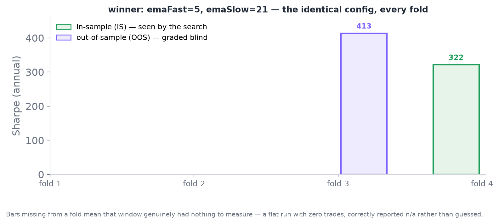Figure 10.2 — The same emaFast=5, emaSlow=21 won every fold that had anything to measure. A different winner each fold would be the tell that the search was fitting noise, not signal.

Second: notice how many n/a entries are scattered through the table — exactly like fold 3’s own training step, and exactly like Chapter 9’s honest refusal to fabricate a ratio from an undefined denominator. A fold whose window happened to contain no real signal correctly says so, rather than inventing a number to fill the cell.

The curve that’s actually allowed to be trusted#

The harness stitches every fold’s test-only equity curve into one continuous series — never the train curves, which were seen by the search and are exactly what Chapter 9 already warned you not to trust:

internal fun concatenate(curves: List<List<EquitySample>>): List<EquitySample> {
    // preserves each fold's own P&L delta rather than resetting to zero at the boundary,
    // so the stitched curve reads as one continuous account, not four disconnected charts
}

This concatenated curve is the one number in this whole chapter that deserves real trust, because it’s the only one built entirely out of decisions made on data those decisions never got to see. It’s the closest thing a backtest can produce to an honest answer to: if I had actually been running this strategy live, periodically re-optimizing on what I’d already lived through and then trading forward blind, what would really have happened?

What this doesn’t fix#

It would be dishonest to end here without naming the limit. Walk-forward analysis doesn’t prove a strategy is good — it only proves that it survived being tested honestly, more than once, on data it never saw during selection. It’s also genuinely expensive: a full parameter sweep runs once per fold, not once for the whole study, so the computational cost scales with both the size of the parameter grid and the number of folds. And the discipline can still be defeated by a human standing outside the tool entirely — a researcher who runs the whole walk-forward study, doesn’t like the answer, tweaks the strategy’s logic (not just its parameters), and reruns the exact same walk-forward split has just turned the entire study into one more in-sample decision, made in slow motion, by hand. The tool enforces the boundary between train and test inside one run. It cannot enforce discipline on the person deciding what to try next.

Two smaller limits are worth carrying out of this chapter as well, because both are easy to read past. Ranking is a stable sort with no explicit tiebreak, so when configurations score identically — as all six did in the fold walked through by hand, every one tied at zero trades — the winner is whichever appeared first in the list. That’s deterministic, which is the property that matters most, but it means a fold whose winner never traded is reporting list order rather than merit. And the stitched curve skips every training period, so its time axis has holes: the elapsed time along it is shorter than the calendar span of the study. It’s an honest record of decisions made blind, not a picture of an account over a continuous stretch of history.

There’s a revealing asymmetry in what it does warn about, too. Search a very large parameter grid and the harness will tell you the trial count is getting dangerous — that’s the coin-flipping problem from the start of this chapter, and it’s watched for. Run a study with a single fold and nothing objects at all. Four folds, in a chapter about not trusting one short sample, is itself a small number; the machinery that catches you for asking too many questions has nothing to say when you accept an answer built on too little evidence. Both are ways to fool yourself. Only one of them currently trips an alarm.